ANCOVA
Determine main effect while accounting for covariate
1 dependent variable
1 or more independent variables
1 or more covariates
A covariate is a variable that can influence the DV. By adding a covariate, we reduce error/residual in the model.
Set \(\alpha\) before the data
“We propose to change the default P-value threshold for statistical significance from 0.05 to 0.005 for claims of new discoveries.”
Benjamin et al. (2018) : Redefine statistical significance , 72 authors
Data example
Puppy therapy again (lecture 12), but now we also measured how much each person loves puppies.
Dependent variable: Happiness
Independent variable: Dose (#groups \(= k = 3\) )
No puppies (\(n = 9\) )
15 mins (\(n = 8\) )
30 mins (\(n = 13\) )
Covariate: Puppy love (0–7)
Define the model
\[{happiness} = {model} + {error}\]
\({model} = {independent} + {covariate}\) \(\color{white}{model} = {dose} + {puppy \; love}\)
\(\color{white}{model}\)
Linear model with \(k-1\) dummy variables:
\[\hat{y} = b_0 + b_1 {dummy}_1 + b_2 {dummy}_2 + b_3 covar\]
Observed group means
aggregate (happiness ~ dose, data, mean)
        dose happiness
1 No puppies  3.222222
2    15 mins  4.875000
3    30 mins  4.846154
Model fit without covariate
What are the beta coefficients when we fit a model that only has dose as a predictor variable?
<- lm (happiness ~ dose, data); fit.group$ coefficients
(Intercept) dose15 mins dose30 mins
   3.222222    1.652778    1.623932
\(b_{0} = 3.22\)
\(b_{15min} = 1.65\)
Prediction for 15 mins: 3.22 + 1.65 = 4.87
\(b_{30min} = 1.62\)
Prediction for 30 mins: 3.22 + 1.62 = 4.84
Model fit with only covariate
What are the beta coefficients when we fit a model that only has puppylove as predictor variable?
<- lm (happiness ~ puppylove, data); fit.covar$ coefficients
(Intercept)   puppylove
  3.6568758   0.2596796
\(b_{0} = 3.66\)
\(b_{love} = 0.26\)
Model fit with all predictor variables (factor + covariate)
What are the beta coefficients when we fit the full model (i.e., with both predictor variables)?
<- lm (happiness ~ dose + puppylove, data); fit$ coefficients
(Intercept) dose15 mins dose30 mins   puppylove
  1.7891883   1.7856801   2.2248813   0.4160421
\(b_{0} = 1.79\)
\(b_{15min} = 1.79\)
\(b_{30min} = 2.22\)
\(b_{love} = 0.42\)
Predictions of the full model
For someone in the 15 mins group with a score of 4 on puppy love:
<- lm (happiness ~ dose + puppylove, data); fit$ coefficients
(Intercept) dose15 mins dose30 mins   puppylove
  1.7891883   1.7856801   2.2248813   0.4160421
\(b_{0} = 1.79\)
\(b_{15min} = 1.79\)
\(b_{love} = 0.42\)
Prediction for 15 mins: 1.79 + 1.79 + 4 * 0.42 = 5.26
How about someone in the 30 mins group with a score of 1 on puppy love?
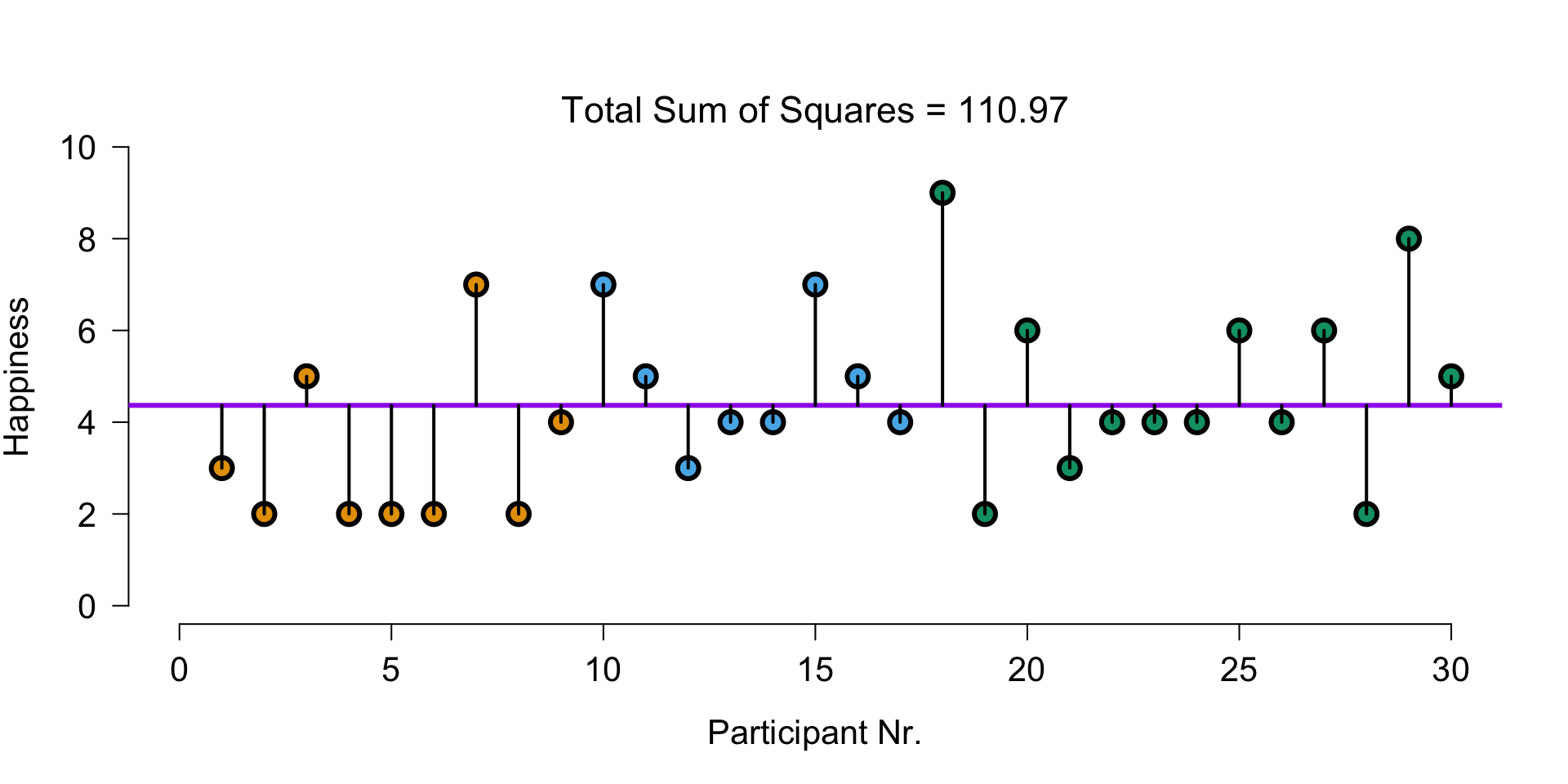
Visual \({SS}_{total}\)
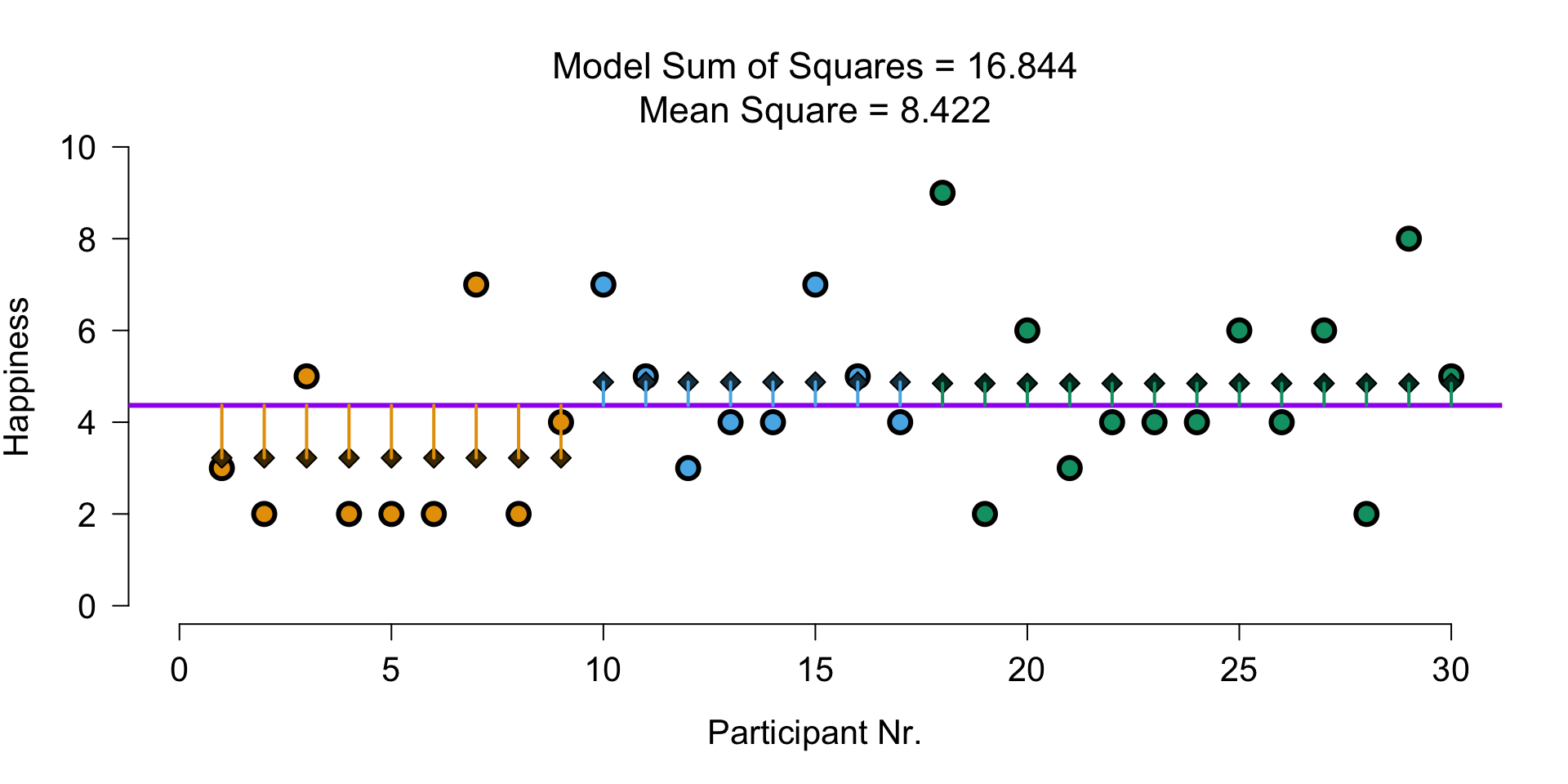
Explained by group model
The model that predicts only using group means:
\(\hat{y} = b_0 + b_1 {dummy}_1 + b_2 {dummy}_2\)
\(\hat{y} = 3.22 + 1.65 \times {dummy}_1 + 1.62 \times {dummy}_2\)
Visual \({SS}_{model}\) : group
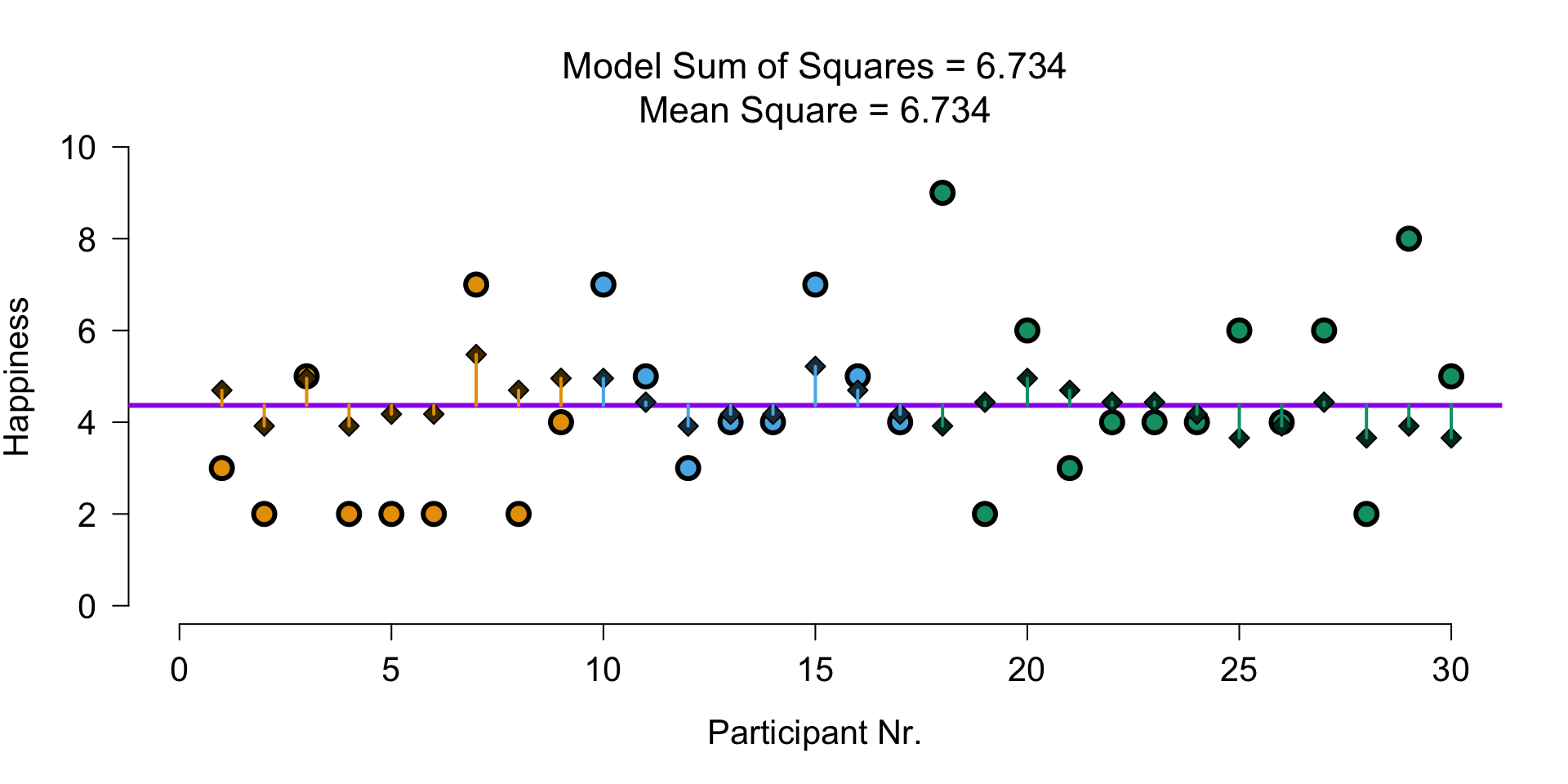
Explained by covariate model
The model that predicts only using puppy love:
\(\hat{y} = b_0 + b_3 covar\)
\(\hat{y} = 3.66 + 0.26 \times {Puppy \; love}\)
Visual \({SS}_{model}\) : covariate
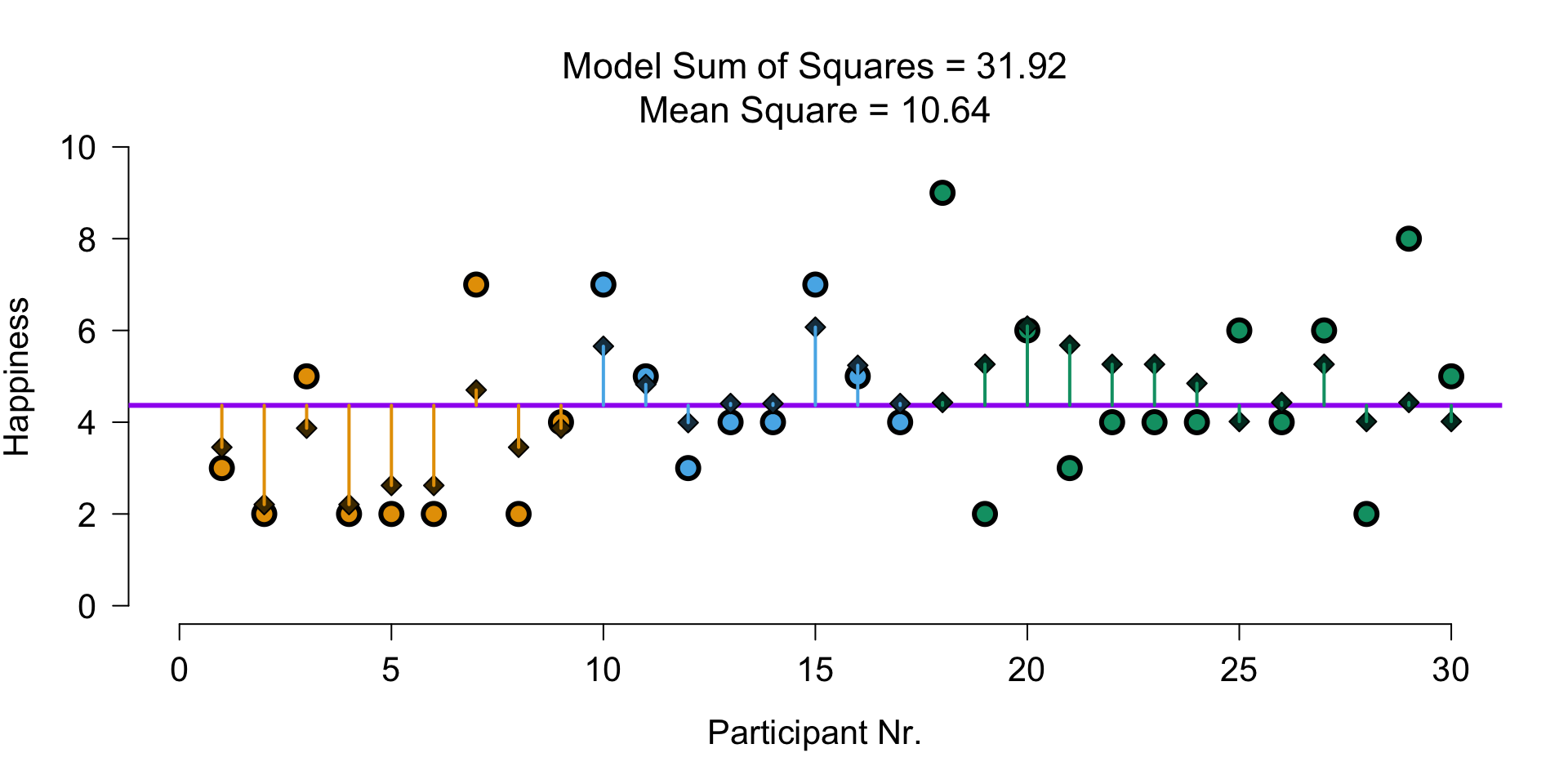
Explained by full model
The model that predicts with group and covariate:
\(\hat{y} = b_0 + b_1 {dummy}_1 + b_2 {dummy}_2 + b_3 covar\)
\(\hat{y} = 1.79 + 1.79 \times {dummy}_1 + 2.22 \times {dummy}_2 + 0.42 \times {Puppy \; love}\)
Visual \({SS}_{model}\) : group + covariate
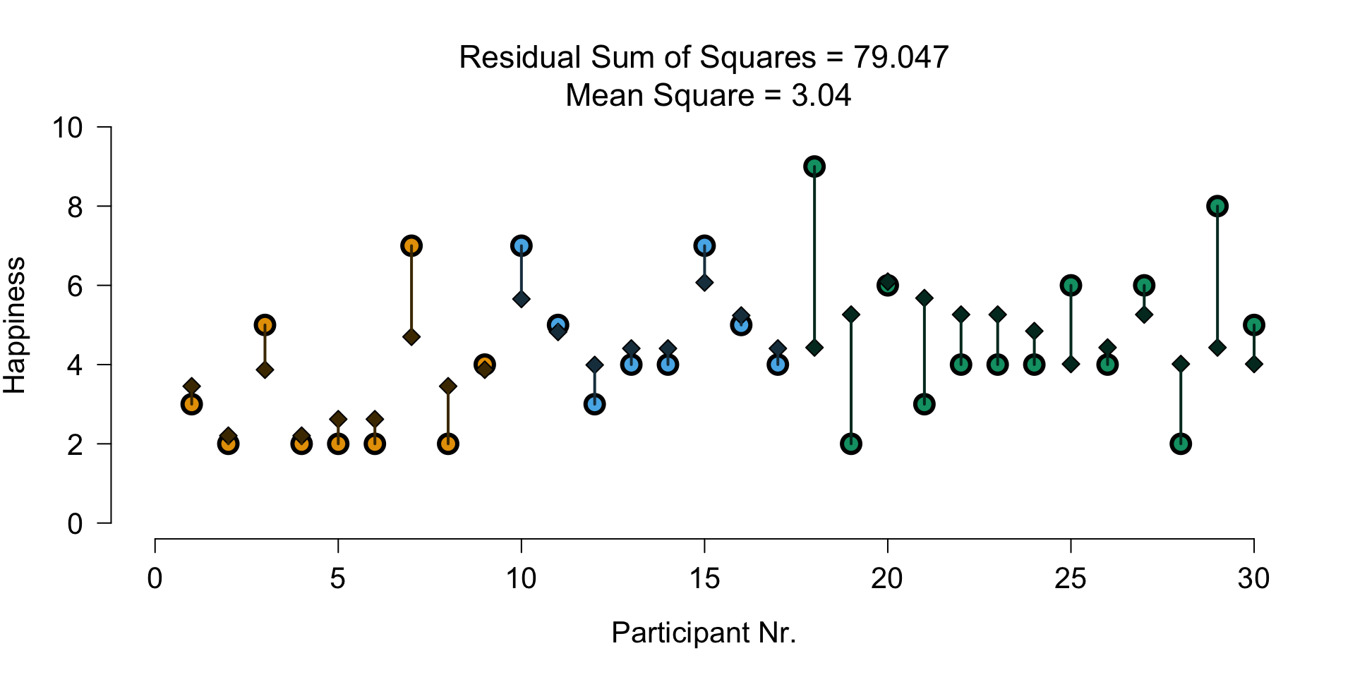
Visual \({SS}_{residual}\) : group + covariate
Divide model sum of squares
Divide model sum of squares
Model SS of full model:
To see what is explained by group, we subtract the Model SS of the covariate model:
<- SS.model - SS.model.covar; SS.group ## SS.group corrected for covar
To see what is explained by covariate, we subtract the Model SS of the group model:
<- SS.model - SS.model.group; SS.covar ## SS.covar corrected for group
Why don’t the parts add up?
Alone (one-predictor model)
16.84
6.73
23.57
Unique (full model minus the other)
25.19
15.08
40.27
Full model
31.92
Usually (redundancy ): alone parts add up to more than the full model, unique parts to less
Here it’s reversed (suppression , p. 340)
The 30-min group loves puppies least, which causes dose and puppy love to suppress each other’s effect
F-ratio
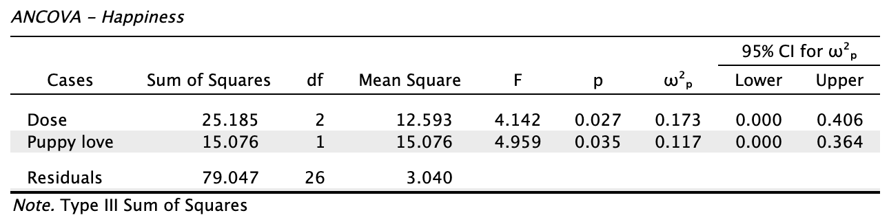
\(MS_{model-group} = \frac{25.185}{2} = 12.593\)
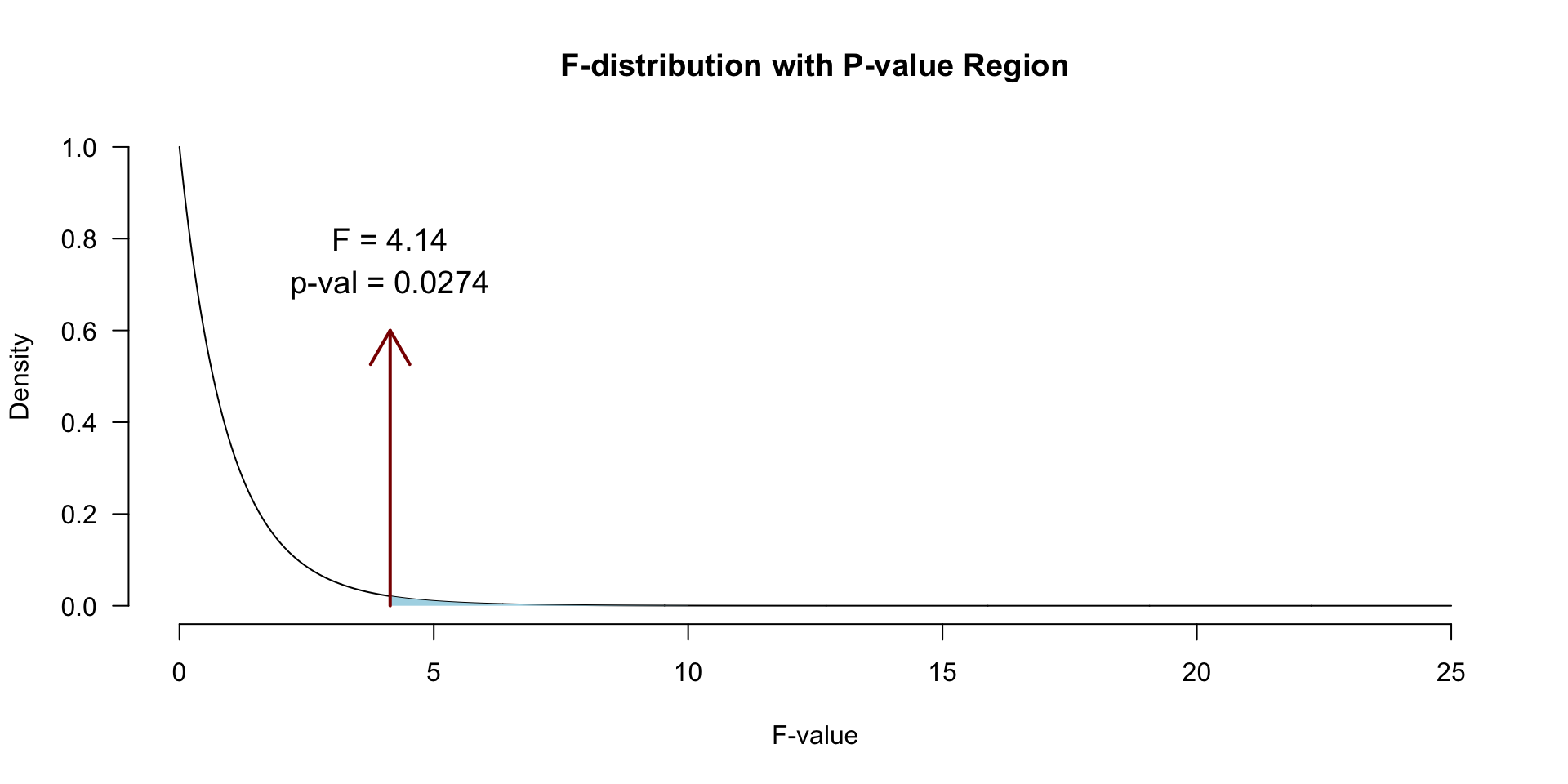
\(F = \frac{{MS}_{model-group}}{{MS}_{residual}} = \frac{{SIGNAL}}{{NOISE}} = \frac{12.593}{3.04} = 4.14\)
\(p\) -value
What if we ignore puppy love?
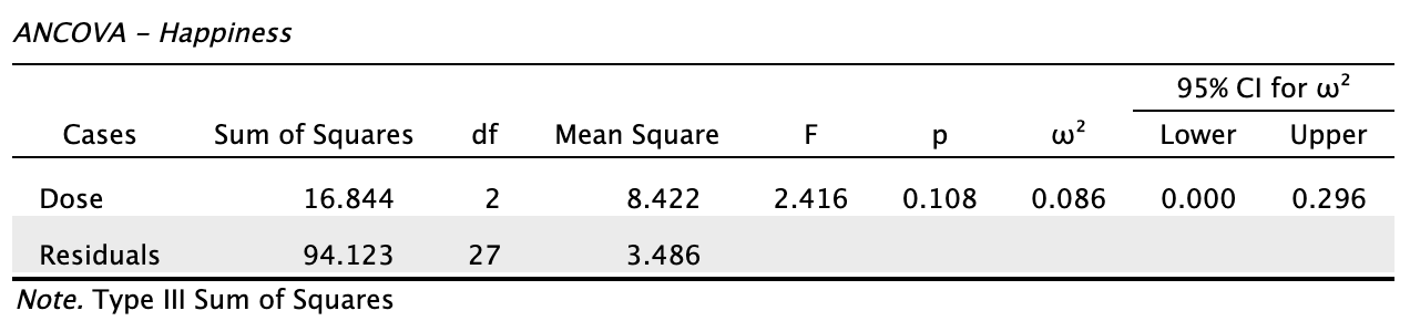
Without puppy love (Output 12.4):
With puppy love (Output 12.5):
\({SS}_{residual}\) : 94.12 → 79.05; effect of dose: \(p\) = 0.108 → \(p\) = 0.027 (§12.7)
Alpha & Power
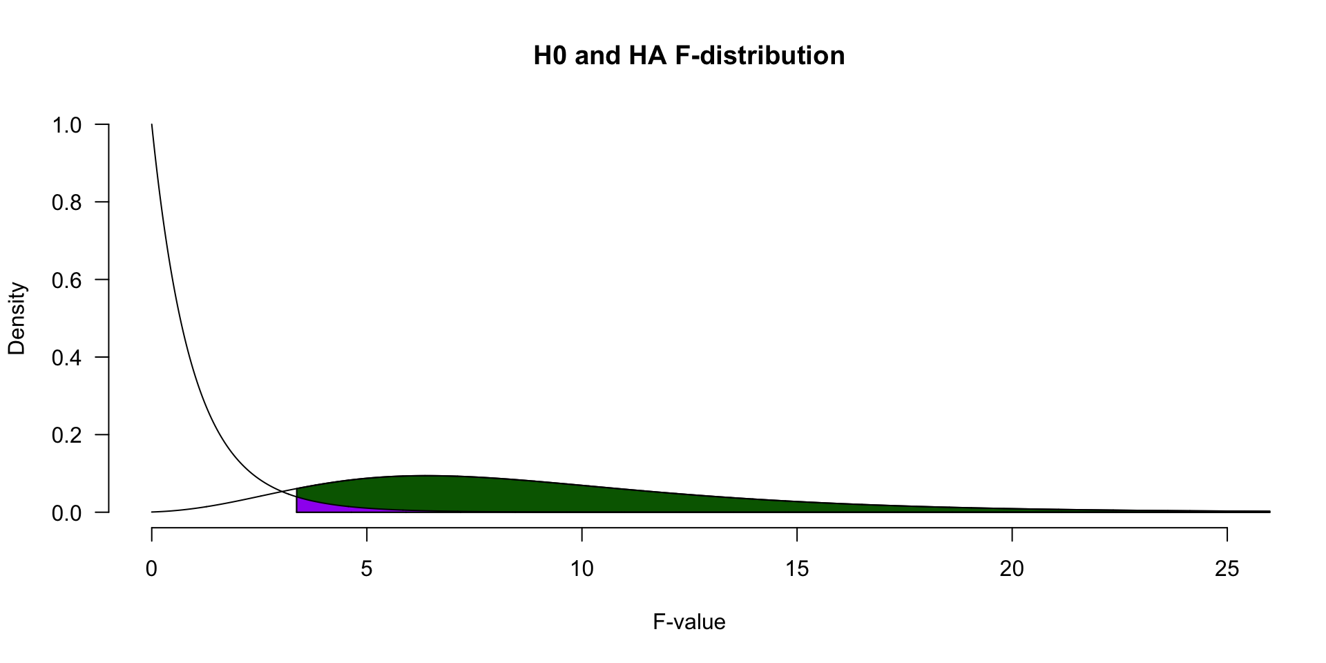
Power becomes quite abstract when we increase the complexity (i.e., number of predictors) of our models. We can make an F-distribution that symbolizes the alternative distribution by shifting the distribution more to the right (although the interpretability becomes pretty murky..)
Adjusted/marginal means
Marginal means are estimated group means, while keeping the covariate equal across the groups
What are happiness averages in each group, if they would all score the same on puppy love?
See also this blogpost
Adjusted/marginal means
Adjusted:
        dose mean.adj
1 No puppies 2.926370
2    15 mins 4.712050
3    30 mins 5.151251
Observed:
        dose happiness
1 No puppies  3.222222
2    15 mins  4.875000
3    30 mins  4.846154
Assumptions
Same as ANOVA
Independence of the covariate and treatment effect §12.5.1.
No difference on ANOVA with covar and independent variable
Matching experimental groups on the covariate
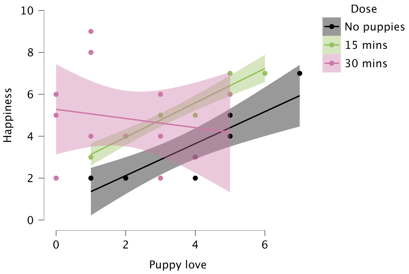
Homogeneity of regression slopes §12.5.2.
Visual: scatterplot dep var * covar per condition
Testing: interaction indep. var * covar
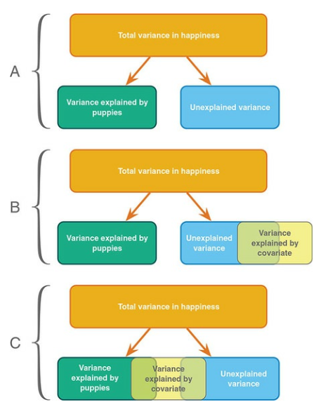
Independence of the covariate and treatment effect (Fig 12.2)
Independence of the covariate
Groups should not differ on the covariate (§12.5.1)
Otherwise: covariate and group share variance (Fig 12.2C)
Associated predictors can inflate/deflate the group effect (F, adjusted means)
Does not “control for” the group difference
Interpretation problem, not a statistical requirement (Jane Superbrain Box 12.1)
Risk mostly without random assignment
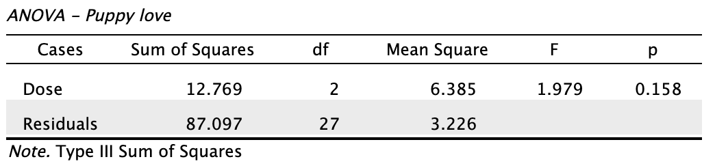
Assess: ANOVA with covariate as dependent variable (§12.6.3)
ANOVA on puppy love: F(2, 27) = 1.98, p = 0.158
Homogeneity of regression slopes
One slope for the covariate: parallel lines (§12.5.2)
Assumes the same covariate-DV relation in every group
Unequal slopes:
Interpretation: effect of dose depends on puppy love (§12.8)
Inflated Type I error (Jane Superbrain Box 12.2)
Assess: add the interaction dose * puppy love to the model (§12.8)
Descriptives plot: are the lines per group roughly parallel?
What does “dose” mean here?
0
0.59
2.31
5.28
0.003
2.73 (average)
2.68
4.55
4.69
0.025
5
4.41
6.41
4.19
0.138
Each dose has its own slope, so the dose effect depends on puppy love
In the model with the interaction, “Dose” compares the groups at puppy love = 0
Interaction present: little value in interpreting the main effect (p. 568)
JASP